Handling Spatial Projection & CRS in R

Authors
Joseph Stachelek, Leah Wasser, Megan A. Jones

Overview

Teaching: 10 min
Exercises: 0 min

Questions

What to do when vector data don’t line up.

Objectives

Know how to identify the CRS of a spatial dataset.

Be familiar with geographic vs. projected coordinate reference systems.

Be familiar with the proj4 string format which is one format used used to store / reference the CRS of a spatial object.

Things You’ll Need To Complete This Tutorial

R Skill Level: Intermediate - you’ve got the basics of R down. You will need the most current version of R and, preferably, RStudio loaded on your computer to complete this tutorial.

Install R Packages

raster: install.packages("raster")

sf: install.packages("sf")

More on Packages in R - Adapted from Software Carpentry.

Data to Download

Site layout shapefiles

In this tutorial, we will create a base map of our study site using a United States state and country boundary accessed from the United States Census Bureau. We will learn how to map vector data that are in different CRS and thus don’t line up on a map.

Working With Spatial Data From Different Sources

To support a project, we often need to gather spatial datasets for from different sources and/or data that cover different spatial extents. Spatial data from different sources and that cover different extents are often in different Coordinate Reference Systems (CRS).

Some reasons for data being in different CRS include:

The data are stored in a particular CRS convention used by the data provider which might be a federal agency, or a state planning office.
The data are stored in a particular CRS that is customized to a region. For instance, many states prefer to use a State Plane projection customized for that state.

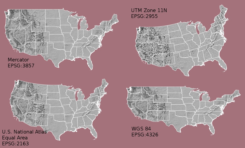
Maps of the United States using data in different projections. Notice the differences in shape associated with each different projection. These differences are a direct result of the calculations used to "flatten" the data onto a 2-dimensional map. Often data are stored purposefully in a particular projection that optimizes the relative shape and size of surrounding geographic boundaries (states, counties, countries, etc). Source: opennews.org

Check out this short video highlighting how map projections can make continents seems proportionally larger or smaller than they actually are!

In this tutorial we will learn how to identify and manage spatial data in different projections. We will learn how to reproject the data so that they are in the same projection to support plotting / mapping. Note that these skills are also required for any geoprocessing / spatial analysis. Data need to be in the same CRS to ensure accurate results.

We will use the sf and raster packages in this tutorial.

# load packages
library(sf)  # for vector work

Linking to GEOS 3.5.0, GDAL 2.2.2, proj.4 4.8.0

library(raster)   # for raster metadata/attributes

Loading required package: sp

# set working directory to data folder
# setwd("pathToDirHere")

Import US Boundaries - Census Data

There are many good sources of boundary base layers that we can use to create a basemap. Some R packages even have these base layers built in to support quick and efficient mapping. In this tutorial, we will use boundary layers for the United States, provided by the United States Census Bureau.

It is useful to have shapefiles to work with because we can add additional attributes to them if need be - for project specific mapping.

Read US Boundary File

We will use the st_read() function to import the /US-Boundary-Layers/US-State-Boundaries-Census-2014 layer into R. This layer contains the boundaries of all continental states in the U.S. Please note that these data have been modified and reprojected from the original data downloaded from the Census website to support the learning goals of this tutorial.

# Read the .csv file
state_boundary_US <- st_read("data/NEON-DS-Site-Layout-Files/US-Boundary-Layers/US-State-Boundaries-Census-2014.shp")

Reading layer `US-State-Boundaries-Census-2014' from data source `/home/travis/build/datacarpentry/r-raster-vector-geospatial/_episodes_rmd/data/NEON-DS-Site-Layout-Files/US-Boundary-Layers/US-State-Boundaries-Census-2014.shp' using driver `ESRI Shapefile'
Simple feature collection with 58 features and 10 fields
geometry type:  MULTIPOLYGON
dimension:      XYZ
bbox:           xmin: -124.7258 ymin: 24.49813 xmax: -66.9499 ymax: 49.38436
epsg (SRID):    4326
proj4string:    +proj=longlat +datum=WGS84 +no_defs

Next, let’s plot the U.S. states data.

# view column names
plot(state_boundary_US$geometry,
     main = "Map of Continental US State Boundaries\n US Census Bureau Data")

plot of chunk find-coordinates

U.S. Boundary Layer

We can add a boundary layer of the United States to our map - to make it look nicer. We will import NEON-DS-Site-Layout-Files/US-Boundary-Layers/US-Boundary-Dissolved-States. If we specify a thicker line width using lwd = 4 for the border layer, it will make our map pop!

# Read the .csv file
country_boundary_US <- st_read("data/NEON-DS-Site-Layout-Files/US-Boundary-Layers/US-Boundary-Dissolved-States.shp")

Reading layer `US-Boundary-Dissolved-States' from data source `/home/travis/build/datacarpentry/r-raster-vector-geospatial/_episodes_rmd/data/NEON-DS-Site-Layout-Files/US-Boundary-Layers/US-Boundary-Dissolved-States.shp' using driver `ESRI Shapefile'
Simple feature collection with 1 feature and 9 fields
geometry type:  MULTIPOLYGON
dimension:      XYZ
bbox:           xmin: -124.7258 ymin: 24.49813 xmax: -66.9499 ymax: 49.38436
epsg (SRID):    4326
proj4string:    +proj=longlat +datum=WGS84 +no_defs

plot(state_boundary_US$geometry,
     main = "Map of Continental US State Boundaries\n US Census Bureau Data",
     border = "gray40")

plot(country_boundary_US$geometry,
     lwd = 4,
     border = "gray18",
     add = TRUE)

plot of chunk check-out-coordinates

Next, let’s add the location of a flux tower where our study area is. As we are adding these layers, take note of the class of each object.

# Import a point shapefile
point_HARV <- st_read("data/NEON-DS-Site-Layout-Files/HARV/HARVtower_UTM18N.shp")

Reading layer `HARVtower_UTM18N' from data source `/home/travis/build/datacarpentry/r-raster-vector-geospatial/_episodes_rmd/data/NEON-DS-Site-Layout-Files/HARV/HARVtower_UTM18N.shp' using driver `ESRI Shapefile'
Simple feature collection with 1 feature and 14 fields
geometry type:  POINT
dimension:      XY
bbox:           xmin: 732183.2 ymin: 4713265 xmax: 732183.2 ymax: 4713265
epsg (SRID):    32618
proj4string:    +proj=utm +zone=18 +datum=WGS84 +units=m +no_defs

# plot point - looks ok?
plot(point_HARV$geometry,
     pch = 19,
     col = "purple",
     main = "Harvard Fisher Tower Location")

plot of chunk explore-units

The plot above demonstrates that the tower point location data is readable and will plot! Let’s next add it as a layer on top of the U.S. states and boundary layers in our basemap plot.

# plot state boundaries
plot(state_boundary_US$geometry,
     main = "Map of Continental US State Boundaries \n with Tower Location",
     border = "gray40")

# add US border outline
plot(country_boundary_US$geometry,
     lwd = 4,
     border = "gray18",
     add = TRUE)

# add point tower location
plot(point_HARV$geometry,
     pch = 19,
     col = "purple",
     add = TRUE)

plot of chunk layer-point-on-states

What do you notice about the resultant plot? Do you see the tower location in purple in the Massachusetts area? No! What went wrong?

Let’s check out the CRS (st_crs()) of both datasets to see if we can identify any issues that might cause the point location to not plot properly on top of our U.S. boundary layers.

# view CRS of our site data
st_crs(point_HARV)

Coordinate Reference System:
  EPSG: 32618 
  proj4string: "+proj=utm +zone=18 +datum=WGS84 +units=m +no_defs"

# view crs of census data
st_crs(state_boundary_US)

Coordinate Reference System:
  EPSG: 4326 
  proj4string: "+proj=longlat +datum=WGS84 +no_defs"

st_crs(country_boundary_US)

Coordinate Reference System:
  EPSG: 4326 
  proj4string: "+proj=longlat +datum=WGS84 +no_defs"

It looks like our data are in different CRS. We can tell this by looking at the CRS strings in proj4 format.

Understanding CRS in Proj4 Format

The CRS for our data are given to us by R in proj4 format. Let’s break down the pieces of proj4 string. The string contains all of the individual CRS elements that R or another GIS might need. Each element is specified with a + sign, similar to how a .csv file is delimited or broken up by a ,. After each + we see the CRS element being defined. For example projection (proj=) and datum (datum=).

UTM Proj4 String

Our project string for point_HARV specifies the UTM projection as follows:

+proj=utm +zone=18 +datum=WGS84 +units=m +no_defs +ellps=WGS84 +towgs84=0,0,0

proj=utm: the projection is UTM, UTM has several zones.
zone=18: the zone is 18
datum=WGS84: the datum WGS84 (the datum refers to the 0,0 reference for the coordinate system used in the projection)
units=m: the units for the coordinates are in METERS.
ellps=WGS84: the ellipsoid (how the earth’s roundness is calculated) for the data is WGS84

Note that the zone is unique to the UTM projection. Not all CRS will have a zone.

Geographic (lat / long) Proj4 String

Our project string for state_boundary_US and country_boundary_US specifies the lat/long projection as follows:

+proj=longlat +datum=WGS84 +no_defs +ellps=WGS84 +towgs84=0,0,0

proj=longlat: the data are in a geographic (latitude and longitude) coordinate system
datum=WGS84: the datum WGS84 (the datum refers to the 0,0 reference for the coordinate system used in the projection)
ellps=WGS84: the ellipsoid (how the earth’s roundness is calculated) is WGS84

Note that there are no specified units above. This is because this geographic coordinate reference system is in latitude and longitude which is most often recorded in Decimal Degrees.

Data Tip

the last portion of each proj4 string is +towgs84=0,0,0 . This is a conversion factor that is used if a datum conversion is required. We will not deal with datums in this tutorial series.

CRS Units - View Object Extent

Next, let’s view the extent or spatial coverage for the point_HARV spatial object compared to the state_boundary_US object.

# extent for HARV in UTM
st_bbox(point_HARV)

     xmin      ymin      xmax      ymax 
 732183.2 4713265.0  732183.2 4713265.0 

# extent for object in geographic
st_bbox(state_boundary_US)

      xmin       ymin       xmax       ymax 
-124.72584   24.49813  -66.94989   49.38436 

Note the difference in the units for each object. The extent for state_boundary_US is in latitude and longitude which yields smaller numbers representing decimal degree units. Our tower location point is in UTM, is represented in meters.

Proj4 & CRS Resources

More information on the proj4 format.
A fairly comprehensive list of CRS by format.
To view a list of datum conversion factors type: projInfo(type = "datum") into the R console.

Reproject Vector Data

Now we know our data are in different CRS. To address this, we have to modify or reproject the data so they are all in the same CRS. We can use st_transform() function to reproject our data. When we reproject the data, we specify the CRS that we wish to transform our data to. This CRS contains the datum, units and other information that R needs to reproject our data.

The st_transform() function requires two inputs:

the name of the object that you wish to transform
the CRS that you wish to transform that object too. In this case we can use the st_crs() of the state_boundary_US object as follows: st_crs(state_boundary_US)

Data Tip

st_transform() will only work if your original spatial object has a CRS assigned to it AND if that CRS is the correct CRS!

Next, let’s reproject our point layer into the geographic - latitude and longitude WGS84 coordinate reference system (CRS).

# reproject data
point_HARV_WGS84 <- st_transform(point_HARV,
                                st_crs(state_boundary_US))

# what is the CRS of the new object
st_crs(point_HARV_WGS84)

Coordinate Reference System:
  EPSG: 4326 
  proj4string: "+proj=longlat +datum=WGS84 +no_defs"

# does the extent look like decimal degrees?
st_bbox(point_HARV_WGS84)

     xmin      ymin      xmax      ymax 
-72.17266  42.53690 -72.17266  42.53690 

Once our data are reprojected, we can try to plot again.

# plot state boundaries
plot(state_boundary_US$geometry,
     main = "Map of Continental US State Boundaries\n With Fisher Tower Location",
     border = "gray40")

# add US border outline
plot(country_boundary_US$geometry,
     lwd = 4,
     border = "gray18",
     add = TRUE)

# add point tower location
plot(point_HARV_WGS84$geometry,
     pch = 19,
     col = "purple",
     add = TRUE)

plot of chunk plot-again

Reprojecting our data ensured that things line up on our map! It will also allow us to perform any required geoprocessing (spatial calculations / transformations) on our data.

Challenge - Reproject Spatial Data

Create a map of the North Eastern United States as follows:

Import and plot Boundary-US-State-NEast.shp. Adjust line width as necessary.
Reproject the layer into UTM zone 18 north.
Layer the Fisher Tower point location point_HARV on top of the above plot.
Add a title to your plot.
Add a legend to your plot that shows both the state boundary (line) and the Tower location point.

Answers

# import mass boundary layer
# read the .csv file
NE.States.Boundary.US <- st_read("data/NEON-DS-Site-Layout-Files/US-Boundary-Layers/Boundary-US-State-NEast.shp")
# view crs
st_crs(NE.States.Boundary.US)

# create CRS object
UTM_CRS <- st_crs(point_HARV)
UTM_CRS

# reproject line and point data
NE.States.Boundary.US.UTM  <- st_transform(NE.States.Boundary.US,
                                UTM_CRS)
NE.States.Boundary.US.UTM

# plot state boundaries
plot(NE.States.Boundary.US.UTM$geometry,
     main = "Map of Northeastern US\n With Fisher Tower Location - UTM Zone 18N",
     border="gray18",
     lwd = 2)

# add point tower location
plot(point_HARV$geometry,
     pch = 19,
     col = "purple",
     add = TRUE)

# add legend
# to create a custom legend, we need to fake it
legend("bottomright",
       legend = c("State Boundary", "Fisher Tower"),
       lty = c(1, NA),
       pch = c(NA, 19),
       col = c("gray18", "purple"),
       bty = "n")

plot of chunk challenge-code-MASS-Map

Key Points

previous episode

Intro to Geospatial Data with R

next episode

Handling Spatial Projection & CRS in R

Authors

Overview

Things You’ll Need To Complete This Tutorial

Install R Packages

Data to Download

Working With Spatial Data From Different Sources

Import US Boundaries - Census Data

Read US Boundary File

U.S. Boundary Layer

Understanding CRS in Proj4 Format

UTM Proj4 String

Geographic (lat / long) Proj4 String

Data Tip

CRS Units - View Object Extent

Proj4 & CRS Resources

Reproject Vector Data

Data Tip

Challenge - Reproject Spatial Data

Answers

Key Points

previous episode

next episode